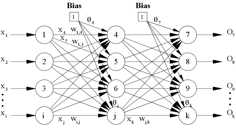
A feedforward neural network is an neural network where connections between layers are in one direction.
The outputs of a layer become inputs (x) to the next.
Coincidentally, matrix math also establishes a one-way relationship.
Consider the following, which multiplies a layer by its weights that map to the next layer.
f \left(
\underbrace{\begin{bmatrix}
1 & x_{i,1} & \cdots & x_{i,n}
\end{bmatrix}_{(1 \times (n+1))}}_{layer_{i}}
\cdot
\underbrace{\begin{bmatrix}
w_{0,0} & \cdots & w_{0,m-1} \\
\vdots & \ddots & \vdots \\
w_{n,0} & \cdots & w_{n,m-1}
\end{bmatrix}_{((n+1) \times m)}}_{weights_{i \rightarrow i+1}}
\right)_{(1 \times m)}
=
\underbrace{\begin{bmatrix}
x_{i+1,1} & \cdots & x_{i+1,m}
\end{bmatrix}_{(1\times m)}}_{layer_{i+1}}
The goal of gradient descent is to calculate an update to the weights,
such that the next calculation of the network will result in a lower error when estimating the output.
In other words, we aim to calculate the change in error with respect to a change in weights (allowing us to know how much to change the weights).
\frac{\partial L}{\partial w_{i \rightarrow i+1}}
Since the product of layer times weights is going to be used a lot, we can simplify it by calling it z.
z_{i(1 \times m)}=\underbrace{\begin{bmatrix}
1 & x_{i,1} & \cdots & x_{i,n}
\end{bmatrix}_{(1 \times (n+1))}}_{layer_{i}}
\cdot
\underbrace{\begin{bmatrix}
w_{0,0} & \cdots & w_{0,m-1} \\
\vdots & \ddots & \vdots \\
w_{n,0} & \cdots & w_{n,m-1}
\end{bmatrix}_{((n+1) \times m)}}_{weights_{i \rightarrow i+1}}
This notation can be summarized as follows:
z = x \cdot w
such that we revisit the matrix differentiation rules:
\frac{\partial L}{\partial w} = x^T \frac{\partial L}{\partial z}
\frac{\partial L}{\partial x} = \frac{\partial L}{\partial z}^T \cdot w
\frac{\partial z}{\partial x} = w^T
\frac{\partial z}{\partial w} = x
This is important when we consider the function f(z).
This could be a number of different functions - typically of the sigmoid family.
logistic, hyperbolic tangent, arctangent, etc.
Sigmoid functions range from 0 to 1 across all inputs (not actually reaching 0 or 1 in practice) and are both reversible and differentiable.
One such sigmoid function is the logistic function:
f \left(z \right ) = \frac{1}{1 + e^{-z}}
which can be differentiated as follows
f' \left(z \right ) = \frac{\partial }{\partial z}f(z) = \frac{e^{-z}}{\left(1 + e^{-z} \right )^2}
and expanded
\frac{e^{-z}}{\left(1 + e^{-z} \right )^2} = \frac{1}{1 + e^{-z}} \cdot \frac{e^{-z}}{1 + e^{-z}}
further expands to
\frac{1}{1 + e^{-z}} \cdot \frac{e^{-z}}{1 + e^{-z}} = \frac{1}{1 + e^{-z}} \cdot \left(1 - \frac{1}{1 + e^{-z}} \right)
which simplifies to
\frac{1}{1 + e^{-z}} \cdot \left(1 - \frac{1}{1 + e^{-z}} \right) = f(z) \cdot \left(1- f(z) \right )
such that
f'(z)_{(1 \times m)} = f(z)_{(1 \times m)} * \left(1- f(z) \right )_{(1 \times m)}
where * is the Schur/Hadamard product.
This is the product of each element - not the matrix product.
In the same manner, the logistic function can be inverted using.
f^{-1} \left(z \right ) = ln \left(\frac{1}{z} - 1\right)
This, however, assumes that x never reaches 0 or 1 exactly.
We now think about what the network hopes to minimize, and that is error/residual/loss.
The loss function is often defined as the 1/2 residual sum squared.
L = \frac{1}{2}\cdot \left( \underbrace{\tilde{x}_{(1 \times m)}}_{measured} - \underbrace{\hat{x}_{(1 \times m)}}_{estimated} \right )^2
Such that it can be conveniently differentiated as follows:
\frac{\partial L}{\partial x} = \underbrace{\hat{x}_{(1 \times m)}}_{estimated} - \underbrace{\tilde{x}_{(1 \times m)}}_{measured}
Since we also know that error is driven by the estimates,
\frac{\partial}{\partial z}\hat{x} = \frac{\partial}{\partial z}f(z) = f'(z) = f(z) * (1-f(z))
the chain rule can then be applied
\frac{\partial}{\partial z}L =\frac{\partial L}{\partial \hat{x}} \frac{\partial \hat{x}}{\partial z} =
\left(\underbrace{\hat{x}_{i_{(1 \times m)}}}_{estimated} - \underbrace{\tilde{x}_{i_{(1 \times m)}}}_{measured} \right ) * f'(z_{i-1})_{(1 \times m)}
and substituting in we see
\frac{\partial L}{\partial w_{i \rightarrow i+1}} = x^T_{i} \cdot \frac{\partial L}{\partial z_i}
=
\begin{bmatrix}
1 \\
x_i,1 \\
\vdots \\
x_i,n
\end{bmatrix}_{((n + 1) \times 1)}
\cdot
\begin{bmatrix}
\left(\underbrace{\hat{x}_{i+1,(1 \times m)}}_{estimated} - \underbrace{\tilde{x}_{i+1,(1 \times m)}}_{measured} \right )
*
f' \left(z_i_{(1 \times m)} \right )_{(1 \times m)}
\end{bmatrix}_{(1 \times m)}
=
\begin{bmatrix}
1 \\
x_i,1 \\
\vdots \\
x_i,n
\end{bmatrix}_{((n + 1) \times 1)}
\cdot
\begin{bmatrix}
\left(\underbrace{\hat{x}_{i+1,(1 \times m)}}_{estimated} - \underbrace{\tilde{x}_{i+1,(1 \times m)}}_{measured} \right )
*
f' \left(x_i_{(1 \times (n+1))} \cdot w_{i \rightarrow i+1, ((n+1) \times m)} \right )_{(1 \times m)}
\end{bmatrix}_{(1 \times m)}
The last part is to set a learning rate  such that
\delta w_{i \rightarrow i+1} += \gamma \cdot \frac{\partial L}{\partial w_{i \rightarrow i+1}}
Great, but what about the weights of the previous layers?
First we need to know how L varies with x.
\frac{\partial L}{\partial x_{i}} = \frac{\partial L}{\partial z_{i}} \frac{\partial z_{i}}{\partial x_{i}}
and from the above rules of differentiation
\frac{\partial L}{\partial z_{i}}\frac{\partial z_{i}}{\partial x_{i}} = \frac{\partial L}{\partial z_{i}} \cdot w^T_{i \rightarrow i+1}
Now, again, we can use the chain rule
\frac{\partial L}{\partial w_{i-1 \rightarrow i}} = \frac{\partial L}{\partial x_{i}} \frac{\partial x_i}{\partial w_{i-1 \rightarrow i}}
and we know
\frac{\partial x_i}{\partial w_{i-1 \rightarrow i}} = x^T_{i-1} \cdot \frac{\partial L}{\partial z_{i-1}}
where
\frac{\partial L}{\partial z_{i-1 }} = \frac{\partial L}{\partial x_{i}} * \frac{\partial x_{i}}{\partial w_{i-1 \rightarrow i}} =\frac{\partial L}{\partial x_{i}} * f'(z_{i-1})
so now
\frac{\partial L}{\partial w_{i-1 \rightarrow i}} =
x^T_{i-1} \cdot
\left(
\underbrace{\left(
\left(
\left(\hat{x}_{i+1} - \tilde{x}_{i+1} \right ) * f'(x_i \cdot w_{i \rightarrow i+1}) \right) \cdot w^T_{i \rightarrow i+1}
\right )}_{\frac{\partial L}{\partial x_{i}}} *
f'(x_{i-1} \cdot w_{i-1 \rightarrow i})
\right )
This is what is referred to as back-propagation.
It is performed from the final layer back to the initial layer before the new residual is calculated.