The least squares problem has an analytical solution - achieving a feasible solution when minimized.
Though the general objective is to minimize error, various other strategies have their limitations or simply will not achieve a single feasible solution.
The goal is to create a series of coefficients, x, that can map the inputs, H, to the outputs, y.
\tilde{y}_{m \times 1} = H_{m \times n} \cdot \hat{x}_{n \times 1}
The Least Squares method attempts to minimize the residual in order to achieve best estimates of model parameters which achieves the ”best fit” approximation.
The best fit minimizes the difference from the truth (the error) and how we define this difference is called the residual.
The residual (error) of a prediction is given as follows
r = \underbrace{\tilde{y}}_{\text{measured}}-\underbrace{\hat{y}}_{\text{estimated}} = \tilde{y} - H \cdot \hat{x}
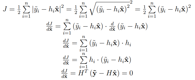
The sum squared of the residual is then found to be
J = \frac{1}{2}\cdot \left( r^T \cdot r \right)
= \frac{1}{2}\cdot \left( \left(\tilde{y} - H \cdot \hat{x} \right )^T \cdot \left(\tilde{y} - H \cdot \hat{x} \right ) \right)
which is rewritten as
J = \frac{1}{2} \cdot \left(
\left(\tilde{y}^T - \left( H \cdot \hat{x}\right )^T \right )
\cdot
\left(\tilde{y} - H \cdot \hat{x} \right )
\right)
and expanded to be written as
J = \frac{1}{2}\cdot \left(
\tilde{y}^T \cdot \tilde{y}
- \tilde{y}^T \cdot \left( H \cdot \hat{x}\right )
- \left( H \cdot \hat{x}\right )^T \cdot \tilde{y}
+ \left( H \cdot \hat{x}\right )^T \cdot \left( H \cdot \hat{x} \right )
\right)
To minimize the residual sum squared, we need to find where the derivative is zero.
\frac{\partial J}{\partial x} = \frac{1}{2}\cdot \left(
\frac{\partial }{\partial x} \tilde{y}^T \cdot \tilde{y}
- \frac{\partial }{\partial x}\tilde{y}^T \cdot \left( H \cdot \hat{x}\right )
- \frac{\partial }{\partial x}\left( H \cdot \hat{x}\right )^T \cdot \tilde{y}
+ \frac{\partial }{\partial x}\left( H \cdot \hat{x}\right )^T \cdot \left( H \cdot \hat{x} \right )
\right) = 0
We can take the derivative of each part, as indicated above.
\frac{\partial }{\partial x} \tilde{y}^T \cdot \tilde{y} = 0
Second part:
\frac{\partial }{\partial x}\tilde{y}^T \cdot \left( H \cdot \hat{x}\right ) =
\frac{\partial }{\partial x}\tilde{y}^T \cdot H \cdot \hat{x} =
\tilde{y}^T \cdot H
Third part:
\frac{\partial }{\partial x}\left( H \cdot \hat{x}\right )^T \cdot \tilde{y} =
\frac{\partial }{\partial x}\hat{x}^T \cdot H\cdot \tilde{y} =
\tilde{y}^T \cdot H^T
Last part:
\frac{\partial }{\partial x}\left( H \cdot \hat{x}\right )^T \cdot \left( H \cdot \hat{x} \right) =
\frac{\partial }{\partial x}\hat{x}^T\cdot H^T \cdot H \cdot \hat{x} =
\hat{x}^T\cdot \left( H^T \cdot H \right )^T + \hat{x}^T\cdot H^T \cdot H
= \hat{x}^T\cdot H^T \cdot H + \hat{x}^T\cdot H^T \cdot H
= 2 \cdot \hat{x}^T\cdot H^T \cdot H
So the final derivative is
\frac{\partial J}{\partial x} = \frac{1}{2}\cdot \left(
- 2 \cdot \tilde{y} \cdot H
+ 2 \cdot H^T \cdot H \cdot \hat{x}\right)
=
H^T \cdot H \cdot \hat{x}
- \tilde{y} \cdot H
Since the first derivative is zero (or should be), we write the equation
\hat{x}^T \cdot H ^T H = \tilde{y}^T \cdot H
We can take the transpose of both sides and both sides will still be equal
\left( \hat{x}^T \cdot H ^T H \right )^T = \left( \tilde{y}^T \cdot H \right )^T
and this simplifies to
H ^T H \cdot \hat{x} = H^T \cdot \tilde{y}
So we can solve for x in following way:
\underbrace{\left(H ^T H \right )^{-1} H ^T H}_1 \cdot \hat{x} = \left(H ^T H \right )^{-1} H^T \cdot \tilde{y}
So finally, the pseudo-inverse is reached
\hat{x} = \left(H ^T H \right )^{-1} H^T \cdot \tilde{y}
If there are more columns than rows, it can also take the form of
\hat{x} = H^T \left(H H ^T\right )^{-1} \cdot \tilde{y}