Gram-Schmidt orthogonalization takes a nonorthogonal set of linearly independent functions and constructs an orthogonal basis over an arbitrary interval.
In other words, given the basis function w_1 ,w_2 ,w_3 , \ldots ,w_n ,
construct orthogonal basis function such that \Phi _1 ,\Phi _2 ,\Phi _3 , \ldots ,\Phi _n
such that span\left\{ {w_i } \right\} = span\left\{ {\Phi _i } \right\}.
The original basis functions, which shall be orthogonalized, are increasing in order, such that polynomial basis is developed.
\left( {\begin{array}{*{20}c}
{w_1 } \\
{w_2 } \\
{w_3 } \\
\vdots \\
{w_n } \\
\end{array}} \right) = \left( {\begin{array}{*{20}c}
1 \\
x \\
{x^2 } \\
\vdots \\
{x^{n - 1} } \\
\end{array}} \right)
First define the inner product as
\left\langle {w,\Phi } \right\rangle = \int\limits_{ - 1}^1 {w\left( x \right)\Phi } \left( x \right)dx
The Gram-Schmidt process takes the general form of
\Phi _n = w_n - \sum\limits_{i = 1}^{n - 1} {\frac{{\left\langle {w_n ,\Phi _i } \right\rangle }}{{\left\langle {\Phi _i ,\Phi _i } \right\rangle }}\Phi _i }
Now we can try the Gram-Schmidt process using the basis functions provided above by hand...
The first team is easy:
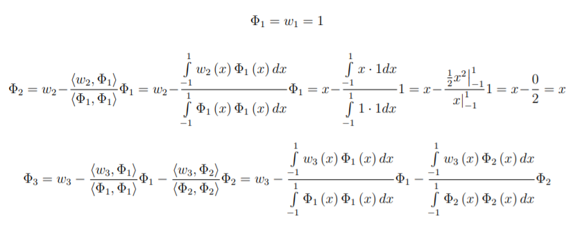
\Phi _1 = w_1 = 1
The second term is a little more complicated, and includes the first term:
\Phi _2 = w_2 - \frac{{\left\langle {w_2 ,\Phi _1 } \right\rangle }}{{\left\langle {\Phi _1 ,\Phi _1 } \right\rangle }}\Phi _1 = w_2 - \frac{{\int\limits_{ - 1}^1 {w_2 \left( x \right)\Phi _1 } \left( x \right)dx}}{{\int\limits_{ - 1}^1 {\Phi _1 \left( x \right)\Phi _1 } \left( x \right)dx}}\Phi _1
= x - \frac{{\int\limits_{ - 1}^1 {x \cdot 1dx} }}{{\int\limits_{ - 1}^1 {1 \cdot 1dx} }}1 = x - \frac{{\left. {\frac{1}{2}x^2 } \right|_{ - 1}^1 }}{{\left. x \right|_{ - 1}^1 }}1 = x - \frac{0}{2} = x
The third term is more involved, as it includes all prior terms:
\Phi _3 = w_3 - \frac{{\left\langle {w_3 ,\Phi _1 } \right\rangle }}{{\left\langle {\Phi _1 ,\Phi _1 } \right\rangle }}\Phi _1 - \frac{{\left\langle {w_3 ,\Phi _2 } \right\rangle }}{{\left\langle {\Phi _2 ,\Phi _2 } \right\rangle }}\Phi _2
\Phi _3 = w_3 - \frac{{\int\limits_{ - 1}^1 {w_3 \left( x \right)\Phi _1 } \left( x \right)dx}}{{\int\limits_{ - 1}^1 {\Phi _1 \left( x \right)\Phi _1 } \left( x \right)dx}}\Phi _1 - \frac{{\int\limits_{ - 1}^1 {w_3 \left( x \right)\Phi _2 } \left( x \right)dx}}{{\int\limits_{ - 1}^1 {\Phi _2 \left( x \right)\Phi _2 } \left( x \right)dx}}\Phi _2
\Phi _3 = x^2 - \frac{{\int\limits_{ - 1}^1 {x^2 \cdot dx} }}{{\int\limits_{ - 1}^1 {1 \cdot 1 \cdot dx} }}1 - \frac{{\int\limits_{ - 1}^1 {x^2 \cdot x \cdot dx} }}{{\int\limits_{ - 1}^1 {x \cdot x \cdot dx} }}x = x^2 - \frac{{\frac{2}{3}}}{2} - \frac{0}{{\frac{2}{3}}}x = x^2 - \frac{1}{3}
This is going to get tedious fast.
This is where Matlab can use symbolic manipulation to get the results.
syms x
n=11; % number of polynomials (order +1)
for p=1:n
    w(p)=x^(p-1);
end

for p=1:n
    phi(p)=w(p);
    if p>1
        for r=1:(p-1)
            phi(p)= phi(p) - int(w(p)*phi(p-r) ,x,-1,1) / int(phi(p-r)*phi(p-r) ,x,-1,1) * phi(p-r);
        end
    end
end

% display the results
phi'
In this example, w can be any pre-defined vector with unique elements.
But, the code in this example produces the following results:
\begin{array}{c}
1 \\
x \\
x^2 - \frac{1}{3} \\
x^3 - \frac{3}{5}x \\
x^4 - \frac{6}{7}x^2 + \frac{3}{{35}} \\
x^5 - \frac{{10}}{9}x^3 + \frac{5}{{21}}x \\
x^6 - \frac{{15}}{{11}}x^4 + \frac{5}{{11}}x^2 - \frac{5}{{231}} \\
x^7 - \frac{{21}}{{13}}x^5 + \frac{{105}}{{143}}x^3 - \frac{{35}}{{429}}x \\
x^8 - \frac{{28}}{{15}}x^6 + \frac{{14}}{{13}}x^4 - \frac{{28}}{{143}}x^2 + \frac{7}{{1287}} \\
x^9 - \frac{{36}}{{17}}x^7 + \frac{{126}}{{85}}x^5 - \frac{{84}}{{221}}x^3 + \frac{{63}}{{2431}}x \\
x^{10} - \frac{{45}}{{19}}x^8 + \frac{{630}}{{323}}x^6 - \frac{{210}}{{323}}x^4 + \frac{{315}}{{4199}}x^2 - \frac{{63}}{{46189}} \\
\end{array}